LLMs Improving LLMs:
Agentic Discovery for Test-Time Scaling
1UMD, 2UVA, 3WUSTL, 4UNC, 5Google, 6Meta
Abstract
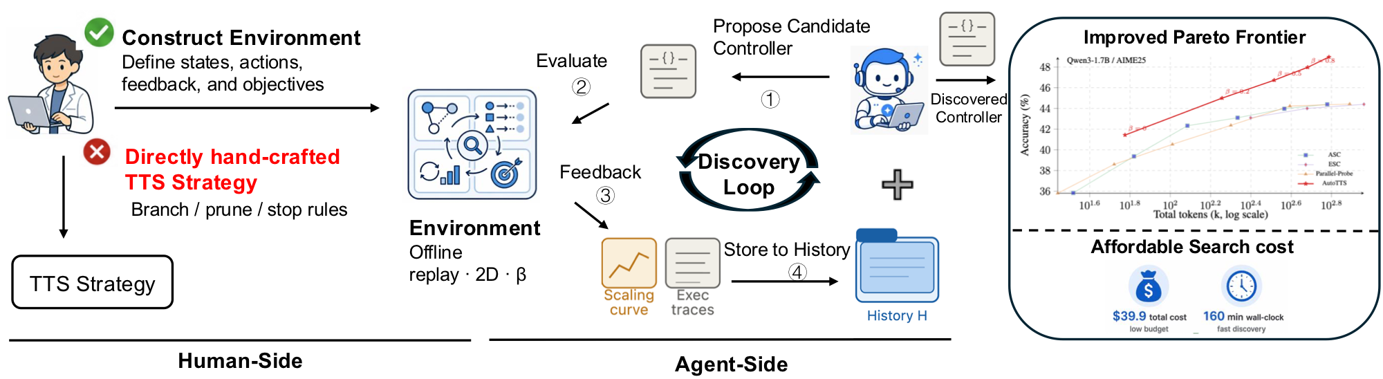
Test-time scaling (TTS) has become an effective approach for improving large language model performance by allocating additional computation during inference. However, existing TTS strategies are largely hand-crafted: researchers manually design reasoning patterns and tune heuristics by intuition, leaving much of the computation-allocation space unexplored.
We propose an environment-driven framework, AutoTTS, that changes what researchers design: from individual TTS heuristics to environments where TTS strategies can be discovered automatically. The key to AutoTTS lies in environment construction: the discovery environment must make the control space tractable and provide cheap, frequent feedback for TTS search.
As a concrete instantiation, we formulate width–depth TTS as controller synthesis over pre-collected reasoning trajectories and probe signals, where controllers decide when to branch, continue, probe, prune, or stop and can be evaluated cheaply without repeated LLM calls. We further introduce beta parameterization to make the search tractable and fine-grained execution trace feedback to improve discovery efficiency by helping the agent diagnose why a TTS program fails.
Experiments on mathematical reasoning benchmarks show that the discovered strategies improve the overall accuracy–cost tradeoff over strong manually designed baselines. The discovered strategies generalize to held-out benchmarks and model scales, while the entire discovery costs only $39.9 and 160 minutes.
Motivation
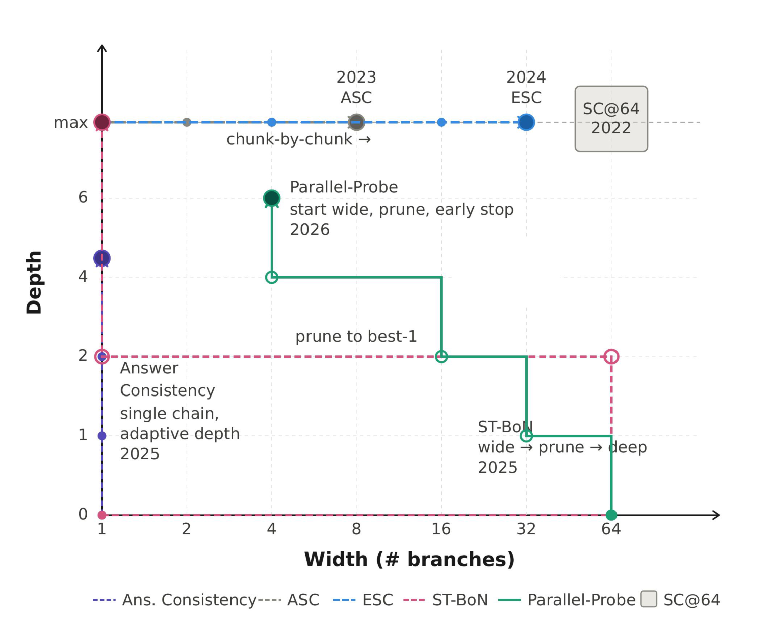
We look back at the trajectory of TTS development. As shown in the figure on the right, many distinct TTS methods can be viewed as special cases in a single shared control space. Take the width–depth view: width = number of parallel branches; depth = how far each branch is extended. If each method is just a point in this space, why keep hand-designing more, instead of treating it as a search problem? This motivates us to rethink the path forward for TTS research: build reusable environments, not more heuristics — define the space, then let a coding agent discover new controllers inside it automatically.
Problem setup
Test-time scaling as algorithmic search
We treat adaptive test-time inference as allocating a finite budget across branches:
open branches, extend them in fixed-length generation intervals, probe to reveal intermediate answers, prune, then aggregate into a final reply—capturing best-of-N, self-consistency, adaptive branching, and related schedules within one formulation.
Branches & probes
Each branch i yields prefixes zi,1, zi,2, …; after each fixed-length interval, an intermediate answer ωi,k exists but enters the controller’s observation only when a probing action is taken.
Budget & cost
Computation is counted in interval units up to budget B.
State cost sums depths plus probing overhead:
Cost(st) = Σi ℓt,i + κprobe·|Ωt| (often κprobe = 0).
State
At step t,
st = (q, mt, It, ℓt, Ωt):
question q,
number of instantiated branches mt,
active branch set It,
depth vector ℓt,
and revealed probe triples Ωt.
Admissible actions
BRANCH— open a new branch through the first interval.CONTINUE(i)— advance branchiby one interval.PROBE(i)— revealωi,ℓwithout advancing depth.PRUNE(i)— deactivatei; depths & past probes stay recorded.ANSWER— terminate and apply aggregation.
Policy, aggregation & objective
A code-defined policy π(· | s, β) maps state s and a scalar meta-parameter β (which deterministically schedules internal knobs) to actions until ANSWER.
The controller may ship its own terminal aggregator Aggπ,β, yielding prediction ŷπ,β(q) and cost Cπ,β(q).
Over tasks (q, y) ~ 𝒟, we maximize accuracy minus penalized cost:
maxπ, β 𝔼q,y[𝟙{ŷπ,β(q) = y} − γ · Cπ,β(q)].
Method
Environment construction before discovery
The MDP of Problem setup is instantiated here as a concrete environment:
fix the interface, pay for base-model forwards once to materialize trajectories, then export a replay table that discovery evaluates without new decoding.
Data collection follows Parallel-Probe: each question receives N independent traces in segments of Δ tokens; all forwards precede the discovery loop.
-
1
Specify the interface
Define state
st, admissible actionsA(st), budget and costCost(st), and the accuracy–cost objective. -
2
Offline trajectory collection
For each query, draw
Nparallel, mutually independent reasoning traces from the backbone (full strings first). Only after this batch completes do we partition each trace into fixed-length segments ofΔtokens and enumerate branch prefixeszi,kwith probe responsesωi,k. -
3
Materialize the replay store
Every environment transition consults the archived table: executing
PROBE(i), for instance, retrieves the archivedωi,kwithout advancing decoding. Repeated scoring passes and sweeps alongβtherefore incur only replay cost. -
4
Hand off to discovery
With the store fixed, candidate controllers are simulated exclusively through
observe/step; asymptotic evaluation cost is dominated by table replay rather than live decoding.
Discovery: β parameterization & trace feedback
Historical records couple offline replay trajectories with search traces; controllers map an external scalar β monotonically into interior hyper-parameters, collapsing outer tuning to a one-dimensional sweep.
Beta parameterization for tractable search
Empirically, automatically generated controllers can introduce on the order of ten coupled hyper-parameters. Across only five outer rounds joint optimization gravitates toward extreme regimes—overly aggressive pruning, for example—that minimize measured tokens on the search benchmark yet fail as generic allocation schedules.
We therefore impose beta parameterization: each artifact exports a lone scalar β together with a deterministic map specifying every internal knob, monotonic so that larger β never reduces the permissible token envelope. Outer search collapses to sweeping β while discouraging brittle thresholds tailored exclusively to Qsearch; in our realization both the programmatic policy and mapping are authored by the coding agent.
History augmentation with execution traces
Scalar summaries such as accuracy or aggregate token totals indicate whether an iteration succeeds but rarely explain systematic failure. Accordingly, alongside each round’s multi-β sweep we archive both empirical scaling curves and the full action-by-action trajectories reconstructed during replay. The former summarizes aggregate quality–budget trade-offs; the latter supplies fine-grained behavioral evidence analogous to tracing harness logs, enabling the explorer to localize defects prior to rewriting code. This design parallels reported gains from execution-level supervision in autonomous software engineering pipelines.
Live case demo
A coding agent refines a controller from grid feedback
This demo replays one held-out AIME25 instance as a 2-D branch-depth grid. Each cell is a cached intermediate answer from the offline environment; the coding agent reads the failure trace, proposes a new OptimalController, evaluates it, appends feedback to history, and uses that history in the next round.
AIME25 · problem 29 · gold answer 104
Propose code, execute on the grid, store feedback, then refine
Five rounds of a coding agent: turn 1 stops too early and returns 196; turns 2–5 rewrite controller.py until the run converges on the gold answer 104.
Repo
Agent reads and edits these files
Claude Code Agent
- ① Read repo history and propose
controller.py - ② Run the controller in
Envon the grid - ③ Inspect trace, vote evidence, tokens, and accuracy
- ④ Store feedback to
Historyfor the next turn
Execution Process
Run the proposed controller on the real AIME25 replay grid.
question
Right triangle ABC, BC = 38, points K,L satisfy AK = AL = BK = CL = KL = 14. Find n if area BKLC = n√3.
actual get_last_trace()
waiting for proposed controller
Press play to execute the current code against cached grid states.
104 correct
196 early trap
ERR
other answer
active this action
visited, not active
pruned / abandoned
final vote evidence
Results
Experimental results
Main results: accuracy & total tokens
-
Setup.
Four Qwen3 backbones; columns report AIME24 (search) plus held-out AIME25/HMMT25 (and averaged held-out where shown).
Higher accuracy and lower cumulative tokens are better; within each backbone block the strongest entry per column is bold.
Rows contrast handcrafted baselines with AutoTTS discovered controllers at two scalar
βsettings. - Trade-offs. Discovered controllers typically achieve a better empirical accuracy–token frontier than the handcrafted methods compared here.
- Generalization. Policies are optimized using only AIME24 replay constructions yet transfer to held-out benchmarks: they outperform every handcrafted baseline on average accuracy for three of four models, and remain competitive on Qwen3-8B (62.7 vs 62.8 for SC@64).
-
β= 0.5. Cuts aggregate token usage by roughly 69.5% vs SC@64 while keeping matched mean held-out accuracy averaged across models (45.3 vs 45.2). -
β= 1.0. Pushes peak accuracy beyond all handcrafted baselines in five of the eight tabulated comparison cells.
| Method | Type | AIME24 (search) | AIME25 (held-out) | HMMT25 (held-out) | Avg. (held-out) | ||||
|---|---|---|---|---|---|---|---|---|---|
| Acc. ↑ | Tokens ↓ | Acc. ↑ | Tokens ↓ | Acc. ↑ | Tokens ↓ | Acc. ↑ | Tokens ↓ | ||
| Base model: Qwen3-0.6B | |||||||||
| SC @ 64 | Handcrafted | 21.4 | 1008.6k | 28.9 | 890.5k | 18.1 | 937.8k | 23.2 | 914.2k |
| ASC | Handcrafted | 21.4 | 805.5k | 28.9 | 653.8k | 18.1 | 580.8k | 23.2 | 617.3k |
| ESC | Handcrafted | 21.4 | 986.7k | 28.9 | 868.8k | 18.1 | 923.9k | 23.2 | 896.4k |
| Parallel-Probe | Handcrafted | 21.8 | 773.8k | 29.7 | 697.8k | 18.5 | 734.5k | 24.1 | 716.2k |
| AutoTTS (β = 0.5) | Discovered | 19.2 | 283.6k | 28.6 | 250.3k | 14.9 | 257.6k | 21.8 | 254.0k |
| AutoTTS (β = 1.0) | Discovered | 20.9 | 542.2k | 31.1 | 474.7k | 18.0 | 487.1k | 24.6 | 480.9k |
| Base model: Qwen3-1.7B | |||||||||
| SC @ 64 | Handcrafted | 72.5 | 1025.8k | 44.4 | 1054.1k | 24.2 | 1132.9k | 34.3 | 1093.5k |
| ASC | Handcrafted | 72.3 | 482.6k | 44.4 | 600.9k | 24.2 | 586.3k | 34.3 | 593.6k |
| ESC | Handcrafted | 72.5 | 909.2k | 44.4 | 913.8k | 24.2 | 1014.2k | 34.3 | 964.3k |
| Parallel-Probe | Handcrafted | 68.1 | 748.5k | 44.7 | 775.8k | 22.6 | 860.2k | 33.7 | 818.0k |
| AutoTTS (β = 0.5) | Discovered | 68.5 | 276.3k | 46.7 | 327.9k | 30.5 | 359.1k | 38.6 | 343.5k |
| AutoTTS (β = 1.0) | Discovered | 70.4 | 499.1k | 49.0 | 612.6k | 32.1 | 679.6k | 40.6 | 646.1k |
| Base model: Qwen3-4B | |||||||||
| SC @ 64 | Handcrafted | 80.0 | 886.8k | 76.6 | 1088.1k | 43.6 | 1168.3k | 60.1 | 1128.2k |
| ASC | Handcrafted | 80.1 | 175.7k | 76.4 | 277.3k | 44.0 | 388.9k | 60.2 | 333.1k |
| ESC | Handcrafted | 80.0 | 528.9k | 76.6 | 793.3k | 43.6 | 990.2k | 60.1 | 891.8k |
| Parallel-Probe | Handcrafted | 79.7 | 688.9k | 76.1 | 806.0k | 44.7 | 872.3k | 60.4 | 839.2k |
| AutoTTS (β = 0.5) | Discovered | 82.0 | 236.7k | 73.8 | 332.3k | 45.7 | 365.0k | 59.8 | 348.7k |
| AutoTTS (β = 1.0) | Discovered | 83.5 | 424.9k | 74.4 | 610.4k | 46.5 | 686.8k | 60.5 | 648.6k |
| Base model: Qwen3-8B | |||||||||
| SC @ 64 | Handcrafted | 80.4 | 910.8k | 76.7 | 1124.4k | 48.9 | 1267.0k | 62.8 | 1195.7k |
| ASC | Handcrafted | 80.4 | 226.0k | 76.7 | 406.2k | 48.8 | 565.1k | 62.8 | 485.7k |
| ESC | Handcrafted | 80.4 | 459.4k | 76.7 | 793.1k | 48.9 | 1062.1k | 62.8 | 927.6k |
| Parallel-Probe | Handcrafted | 81.5 | 730.8k | 76.9 | 846.7k | 47.1 | 897.2k | 62.0 | 872.0k |
| AutoTTS (β = 0.5) | Discovered | 84.3 | 255.3k | 74.1 | 361.2k | 48.1 | 396.7k | 61.1 | 379.0k |
| AutoTTS (β = 1.0) | Discovered | 85.8 | 467.4k | 75.8 | 672.4k | 49.5 | 749.1k | 62.7 | 710.8k |
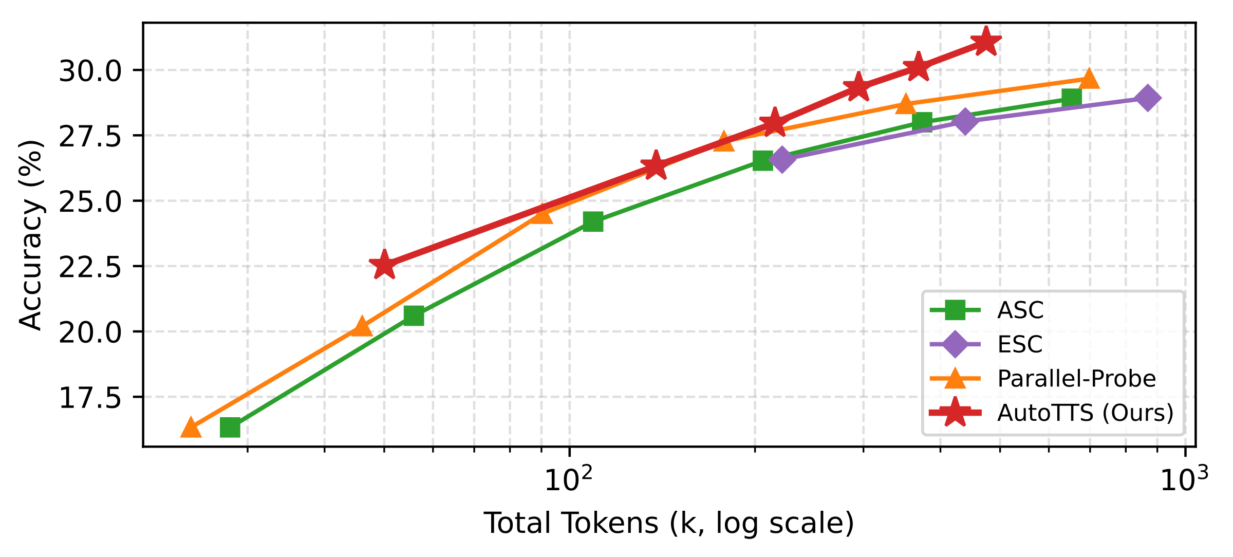
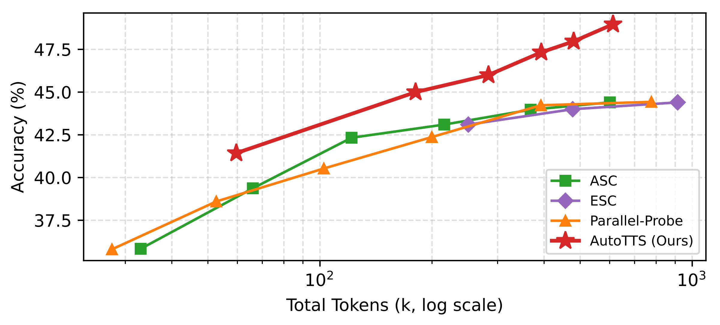
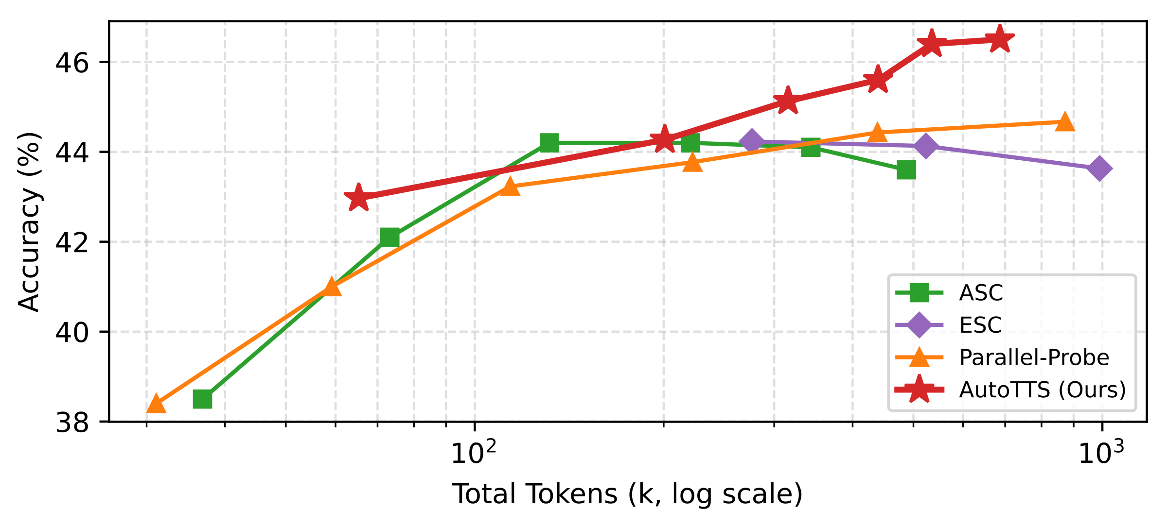
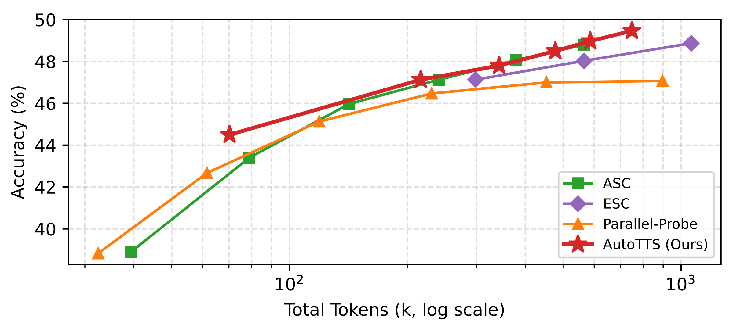
Scaling with β (accuracy vs. tokens)
Sweeping β traces empirical accuracy–token curves against fixed baselines; in each subplot the learned controller shifts toward a better Pareto frontier.
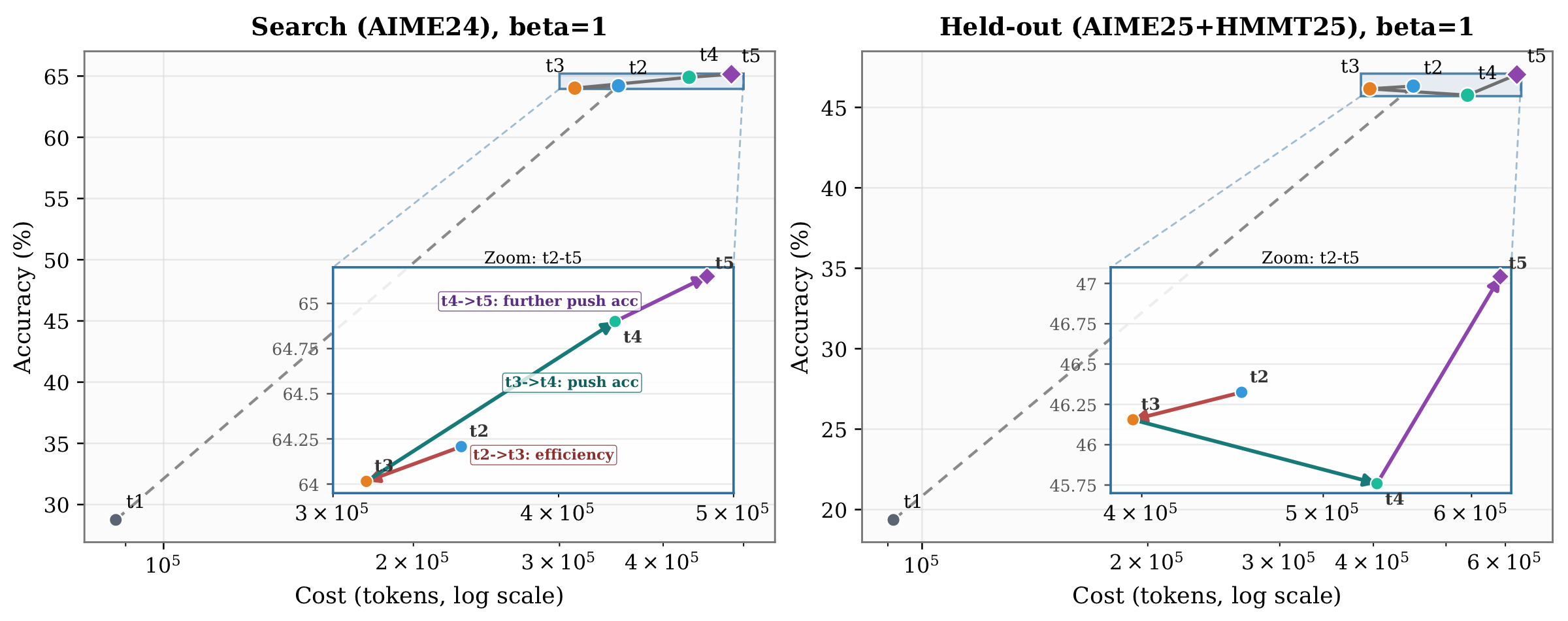
Self-evolving discovery trajectory
Discovery proceeds round by round: each iteration proposes an updated controller from the explorer (Claude Code in our experiments), pushing replay-evaluated accuracy and token cost toward a better accuracy–cost frontier.
Discovered controller
The discovered controller, which we term the Confidence Momentum Controller (CMC), reveals four non-obvious mechanisms.
Trend-based stopping. Rather than gating termination on instantaneous confidence, CMC maintains an EMA of pool confidence and stops only when both the EMA level is high and the trend is non-negative, preventing premature stopping on transient confidence spikes.
Coupled width–depth control. Widening and deepening are linked through the EMA delta: strong confidence gains suppress new branch spawning, while stagnation or regression triggers widening, creating a closed feedback loop absent in all hand-crafted baselines.
Alignment-aware depth allocation.
Each round, branches whose latest answer matches the pool winner receive burst_aligned probe steps. This concentrates computation on the emerging consensus while still advancing all active branches.
Conservative branch abandonment.
A branch is only abandoned after persistently deviating for abandon_patience consecutive rounds, with at least two active branches always preserved.
Together, these mechanisms represent a level of coordinated complexity that would be difficult to arrive at through manual intuition alone.
OptimalController · excerpt
turn_5.py
click to expand
Expand to load source.Citation
@article{zheng2026autotts,
  title = {LLMs Improving LLMs: Agentic Discovery for Test-Time Scaling},
  author = {Zheng, Tong and Liu, Haolin and Huang, Chengsong and Bao, Huiwen and Zhang, Sheng and Liu, Rui and Dai, Runpeng and Chen, Ruibo and Liu, Chenxi and Xiong, Tianyi and Wu, Xidong and Zhang, Hongming and Huang, Heng},
  journal = {arXiv preprint},
  year = {2026}
}
@misc{zheng2026parallelprobe,
title = {Parallel-Probe: Towards Efficient Parallel Thinking via 2D Probing},
author = {Zheng, Tong and Huang, Chengsong and Dai, Runpeng and He, Yun and Liu, Rui and Ni, Xin and Bao, Huiwen and Wang, Kaishen and Zhu, Hongtu and Huang, Jiaxin and Huang, Furong and Huang, Heng},
year = {2026},
eprint = {2602.03845},
archivePrefix = {arXiv},
primaryClass = {cs.CL},
url = {https://arxiv.org/abs/2602.03845},
}